It may sound difficult, but once you’ve mastered using pivot tables, anything is possible. Here are some important tips on how to get the most out of pivot tables in Excel.
Using Dynamic Data Ranges
When you create a pivot table, you use a set range of data (for example, cells A1 to D4). Creating a standard Excel table from your data set before you create a pivot table means that, when you add or remove data, your pivot table should automatically update. This means the information contained within your pivot table will always be accurate. To do this, select a cell in your data set, then press Ctrl+T on your keyboard. Press OK to confirm and create a basic Excel table.
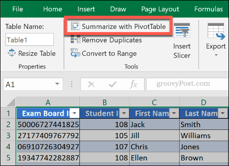
From your new table, you can create a pivot table that will update when the data changes. Click Design > Summarize with PivotTable to do this.
You can then create your Excel Pivot Table as normal, leaving your table as the data range. Set where you wish your pivot table to be created before clicking OK to create it. Once created, add the data fields you wish to see in your pivot table. If your Pivot Table doesn’t update automatically to reflect any changes to your data set, click Analyze > Refresh to manually refresh.
Using Percentage Totals
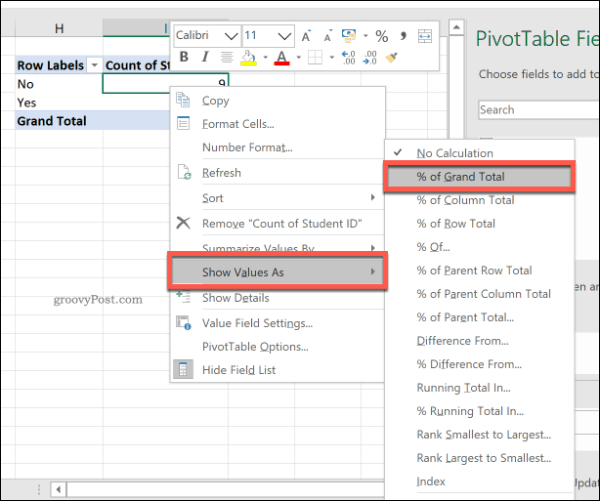
Totals shown in a pivot table will usually be displayed as numbers, but you can change these to percentages. For example, a data set contains information about a group of students, with a column labeled Missed Class which indicates whether or not they’ve ever missed a class. To calculate the percentage of students in this group who have never missed a class, versus the number who have, we could use a percentage total. To do that, right-click on a number in the column you wish to change, then press Show Values As > % of Grand Total.
The updated table will show percentage totals—in this case, 90% for No, 10% for Yes. There are other options, including % of Column Total, if you’d prefer to use these instead.
Renaming Pivot Table Header Labels
When you create a pivot table, headers from your existing data set are used to label a column. When you manipulate your data using SUM or other functions, Excel will usually create a less-than-imaginative header to match the data being manipulated to the function. For our example, calculating the number of students using the Student ID column creates a pivot table header called Count of Student ID. This is somewhat self-explanatory, but the header can still be renamed to make the purpose of this pivot table clearer. To do that, simply edit the header of your pivot table like you would any other cell. Double-click the cell to begin editing it, then replace the text. You can also right-click > Value Field Settings, then type a replacement name in the Custom Name field before clicking OK to save.
Your custom header will remain in place unless (or until) you remove that column from your pivot table.
Using Drill Down in Excel Pivot Tables
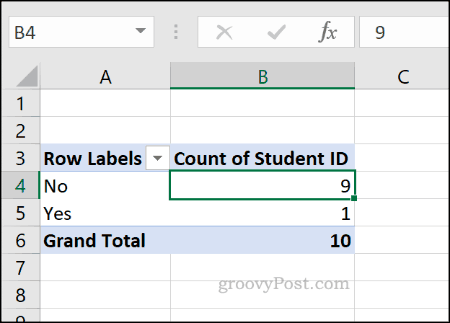
If you have a pivot table containing totals of something, you can drill down to quickly view the information that matches it. For example, in a table that contains the number of students who have missed a class (using our earlier students list data set), we can quickly use this method to view who has (or hasn’t) missed a class.
To do this, double-click on one of your totals. Using the example above, to view all of the students who have missed a class, double-clicking on the total for No (the number 9 in cell B4, in the Count of Student ID column) will display a table with the matching students in a new worksheet.
Changing Cell Number Formatting in Pivot Tables
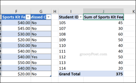
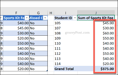
By default, data in your pivot table will appear in the General cell number format. Rather than manually formatting each cell to a different number format, you should set your pivot table to do this instead. For example, an added column to our class list data set called Sports Kit Fee displays the outstanding amount owed by each student for the cost of a sports playing kit, shown in dollars in the original table. Adding this data to a pivot table displays the information in the General cell number format, rather than the correct Currency format.
To change this, right-click on the header label in the pivot table and click Value Field Settings. From there, press the Number Format button. Select Currency from the Format Cells menu before pressing the OK button to save.
The data in your pivot table will update to use your updated cell number formatting. For this example, changing from General to Currency added dollar signs to each value.
Quickly Duplicating Pivot Tables
You don’t have to create a new pivot table each time you want to analyze your data in a slightly different way. If you want to copy a pivot table with custom formatting, for instance, you can simply duplicate the pivot table instead. To do this, click on a cell in your pivot table and press Ctrl+A to select the table as a whole. Right-click and press Copy, or press Ctrl+C on your keyboard. Select an empty cell in another position on your Excel spreadsheet, on the same or different worksheet, then right-click > Paste or press Ctrl+V to paste it.
The new table will be identical to the old table, with the same formatting and data set. You can then modify the pivot table to report different information.
Using Excel for Data Analysis
While pivot tables are useful, they aren’t the only way to analyze data in an Excel spreadsheet. You can concatenate your Excel data to make it easier to understand or use conditional formatting to make certain parts of your data stand out. With these top Excel functions, new users can hit the ground running and start creating advanced Excel spreadsheets, too.


![]()
